
Ever falling, ever missing…
That is an orbit.
What Is An Orbit?
To understand orbits you must first understand motion. In particular, you must understand circular motion and what causes it. Many people think that nothing causes circular motion, and that if an object is moving in a circular path, then it will continue to move in a circular path on its own. Forever.
This is not true.
According to Newton’s First Law of Motion (which was actually discovered by Galileo and later adopted by Newton), an object in motion will continue to move along at a constant speed and with a constant direction unless acted upon by a force. Which is to say that unless something induces an object to change either its speed or its direction, both will stay the same. Forever.
In an orbit, the direction, at least, is constantly changing. So that means that there must be a force acting to maintain the orbital motion, at least according to Newton. To understand how this works, lets first consider the motion of something more down to earth.
Imagine you are swinging an object, perhaps a tennis ball, on the end of a string. Imagine further that the string maintains a constant length, so the tennis ball will move in a circular path. If the speed of the object is constant, then what force is acting on the ball to make it change its direction? The answer is probably fairly obvious: the string pulls it into a circle. If you let go of the string, then the tension in it drops to zero and it no longer exerts a force on the ball. The ball will go flying off in whatever direction it was headed at the moment you let go. If you don’t believe this is true - and a significant number of people do not - I urge you to give this a try. Just make sure you do it in a place where you are not going to knock somebody with your missile when you let go of the string… And make sure you use something light, like a tennis ball, not something heavy, like a rock.
We can understand how this force changes the direction of the object’s motion by applying Newton’s Second Law of Motion.
$$ \vec{F}=m\vec{a} $$
The little arrows above the \(F\) and the \(a\) mean that these quantities, force and acceleration, are vectors. They have both a size (how big is the force, for example) and a direction. What’s more, since the left and right sides of this equation are equal to each other, the force \(\vec{F}\) and acceleration \(\vec{a}\) must point in the same direction because they are the only two vectors present. The mass m has no direction (it is called a scalar), it just scales the acceleration, adjusting its length and converting it into a force.
At this point, if you don’t know what vectors are, or if you are a little bit rusty about how they work, you should have a look at my blog entry on vectors. It’s short and will provide the basic ideas that you will need for this article.
Circular Kinematics
Have a look at the diagram below. It shows an object moving in a circular path. This could be any circular path. Its velocity and acceleration vectors are shown as well.
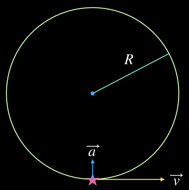
The critical thing to notice in this diagram is that the acceleration vector and the velocity vector are perpendicular to each other. For circular motion this is always true. This is because for circular motion the acceleration points directly at the center of the circle; it is called centripetal acceleration, a fancy name for center-seeking acceleration. Motion along any path is always tangent to the path at whatever point the moving object happens to be. For a circle, a tangent line at any point is always perpendicular to the radial direction, and so the velocity and the centripetal acceleration are always perpendicular. Mathematically, the magnitude of the centripetal acceleration always satisfies the equation below; the variables have the same meanings as in the diagram above, except we have placed a subscript \(c\) to emphasize that the expression refers specifically to centripetal acceleration. This will be important later for understanding the shape of orbits.
$$ a_c=\frac{v^2}{R} $$
From the physics of motion (kinematics) we learn that the acceleration is the change of velocity with time. In fact, this is how acceleration is defined, so it is true for any acceleration from any cause. Mathematically we can write this as follows.
$$ \vec{a}=\frac{\Delta \vec{v}}{\Delta t} $$
The symbol \(\Delta\vec{v}\) represents the change in the velocity that occurs over some time interval \(\Delta t\). Because the velocity is a vector, the change in velocity is also a vector. That means the velocity can change in two ways: it can change its magnitude (the object can speed up or slow down) or it can change its direction. It can also do both, of course, but we will leave that case aside for the moment. For circular orbits, only the direction of the velocity changes. How do we know that? Let’s have a look at the next diagram to begin to understand why that is the case.
In the diagram below, the change in the velocity over some time interval has replaced the acceleration. Both vectors point in the same direction. They must, because they are proportional to each other: to get the change in velocity we simply multiply the acceleration by the scalar quantity \(\Delta t.\) By the way, that should give you some insight into why scalars are given that name - they scale the length of vectors (and convert their units sometimes, too, as here).
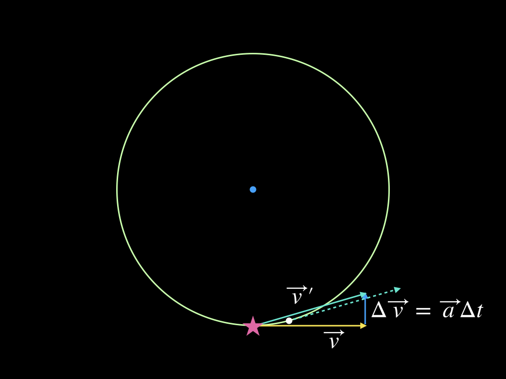
From the diagram above, we know that during the time interval in question, the orbiting object will acquire a new velocity, call it \(\vec{v}^\prime .\) This new velocity is found by adding the change in velocity, \(\Delta \vec{v},\) to the original velocity \(\vec{v}.\) In the diagram, \(\vec{v}^\prime\) is represented by the green arrow.
$$ \vec{v}^\prime=\vec{v}+\Delta \vec{v} $$
In the time required to reach this new velocity, the object will have moved along its orbit to a new position, and this position can be found by parallel transporting the \(\vec{v}^\prime\) vector so as to find the point on the circle where the vector runs tangent to the circular path - keep in mind that we can move vectors around, and as long as we preserve their length and direction they remain the same. This is why we can move \(\vec{v}^\prime\) in the manner described. The intersection of the dotted green vector and the circle shows roughly where the object will be located when it acquires the velocity \(\vec{v}^\prime .\) The point is marked with a white dot.
As an aside, in an actual orbit the velocity is changing all the time, so even over arbitrarily small time intervals there will be (quite small) changes to the velocity, and the orbit is thus a smooth curve, not a disjointed sequence of discrete jumps in velocity as we have implied here.
But how do we know that the speed does not change? Well, for a circular path, the acceleration is always perpendicular to the velocity. That means that there is no amount of acceleration that is in the same direction (or the opposite direction) as the velocity vector. Only such an acceleration component could change the speed; a perpendicular acceleration component can only change the velocity’s direction. If you know how work is defined in physics, then you can think of this in those terms: a force (or acceleration) that is perpendicular to a displacement (or velocity) cannot do any work on an object, and so cannot change the object’s energy (or in other words, change its speed). If you don’t know about the definition of work, then no worries. If you understand the tail-to-head addition rule for vectors, then you can probably convince yourself that the speed of a particle moving in a circle will remain constant if the only acceleration acting on it is the centripetal acceleration.
Orbital Dynamics
The kinematics discussed above are true for any type of circular motion. They are true for a tennis ball swinging with constant speed on a string with constant length, a car traveling around a curve of constant curvature with constant speed, or a satellite moving along a circular orbit at a constant speed. All of these are examples of circular motion, and the relationship between speed, velocity and acceleration will be the same for all of them. However, the causes of those accelerations are quite different for each of these cases, and it is the forces that we turn to now.
In the discussion below we will assume that the central object is much more massive than the orbiting object. This is so we can imagine the central object is essentially stationary as the smaller object travels around it. In fact, both objects orbit about their common center of mass. For a central object that is much more massive, the center of mass of the two nearly coincides with the center of mass of the central object. Under these assumptions only a small error is introduced. So just keep in mind that our treatment assumes a very massive, immobile central object that is orbited by a much less massive “test object.” If you would like to see a more general treatment you should have a look at a text book on orbital dynamics.
As we mentioned already, the force that causes a tennis ball to accelerate inward is the tension acting through he string. The force causing the acceleration of a car around a curve is the friction between the road and its tires. If you doubt this, try turning sometime on an icy road. You will find the exercise fraught with difficulty.
For an orbiting object, which is the primary concern of this article, the force that creates the centripetal acceleration is gravity. That is the force that keeps the planets and other members of the solar system from flying off into space. Gravity also keeps us all from springing up from the ground and flying into the sky. In the Newtonian view, gravity always acts along the line connecting two objects, and it is always attractive. So if we imagine a planet orbiting a star, we will have a diagram just like first one, with the force of gravity providing the centripetal acceleration. We could say that in this case the centripetal acceleration is the gravitational acceleration.
(We usually discuss gravity in terms of the force it exerts, as that force is described by Newton’s Universal Law of Gravitation. In many ways it makes a lot more sense to think of gravity as an acceleration instead of a force. After going through this article, perhaps you will believe that this is a better way to think about gravity too.)
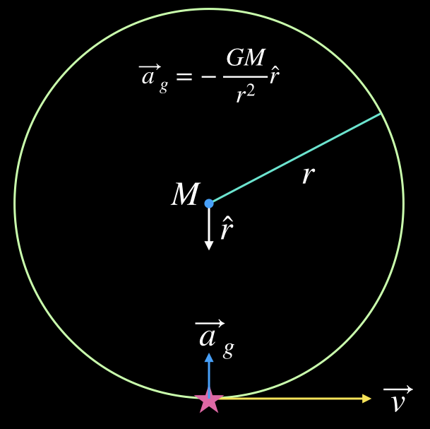
The diagram above has a lot going on. Each of its parts are described below. the centripetal acceleration, which is explicitly given as the gravitational acceleration, \(\vec{a}_g.\) It shows the orbital velocity of the object, \(\vec{v}.\) It also gives the radius of the orbit, \(r\) and the mass of the central object, \(M.\) The symbol \(\hat{r}\) is a radial unit vector: it points in the radial direction, always toward the orbiting object, and it has unit length (a length of one in arbitrary units). It is a mathematical indicator that the gravitational force and acceleration point in the opposite direction of the radius vector, which points from the center of the circle to the orbiting object. Don’t confuse the orbital size, \(r\) with the orbital radius vector \(\vec{r}=r\hat{r}\). The size is shown in the diagram, but \(\vec{r}\) has been left off because showing it would make the diagram more busy than it already is. Just keep in mind, if you like, that \(\vec{r}\) points in the direction of \(\hat{r}\) and has length \(r.\)
- \(\vec{a}_g\) - gravitational acceleration
- \(M\) - object at the center of the orbit, the Sun in the solar system, Earth for the Moon and other satellites.
- \(r\) - the size of the orbit, the orbital radius.
- \(\hat{r}\) - radial unit vector. It always points radially outward from the center of the circle toward the orbiting object. It has unit length (a length of 1 in arbitrary units) and no physical units like meters, inches, feet, etc. It is a mathematical object that tells us that the gravitaitonal force and acceleration act along the radial direction only.
- \(\vec{v}\) - the orbital velocity. Its magnitude, \(v\), is the speed of the orbiting object.
The gravitational acceleration is found by using Newton’s Second Law of Motion along with his Universal Law of Gravitation. Together they give the expression shown above. We demonstrate this below.
Begin with the Law of Gravitation in the first line, then substitute using the Second Law in the second line. We then cancel the common factor of \(m\), the mass of the orbiting object, to arrive at the gravitational acceleration in the third line.
\begin{equation}
\begin{split}
\vec{F}_g &=-\frac{GMm}{r^2}\hat{r}\\
m\vec{a}_g & = -\frac{GMm}{r^2}\hat{r}\\
\vec{a}_g & = -\frac{GM}{r^2}\hat{r}
\end{split}
\end{equation}
The gravitational acceleration is only in the radial direction (it points in the \(-\hat{r}\) direction) and so the object orbits at constant speed, just as we found before for circular motion. Only with gravity we can think a bit more deeply about the motion than we did previously.
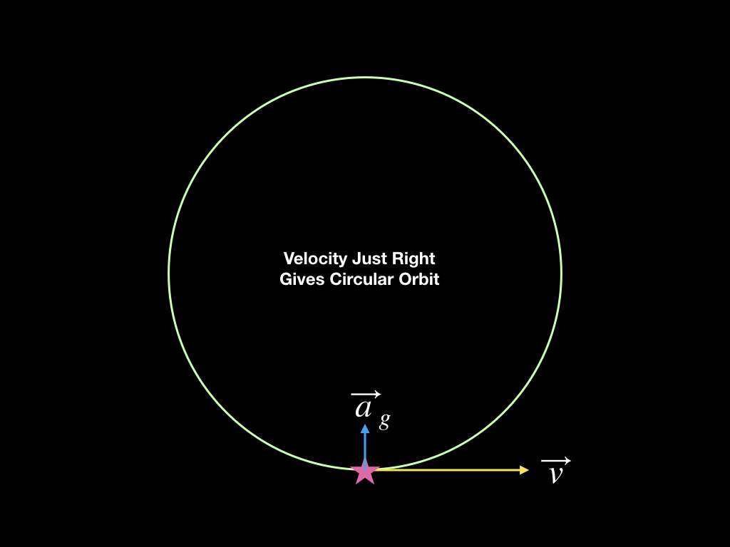
In order for the orbit to be circular, the velocity must be tuned just right. The tendency of the test object to fall toward the center under the influence of gravity must exactly match its tendency to move away from the center provided by its orbital speed. For a given gravitational acceleration there is only a single orbital speed that will satisfy this. It is the speed that you would put into the expression for centripetal acceleration to get the gravitational acceleration that the object feels. Only at this speed will the orbit be a circle. This case is represented in the diagram above.
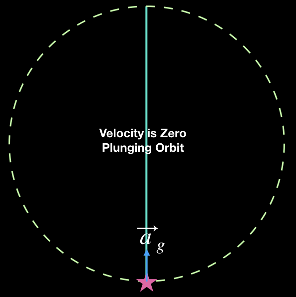
For other speeds, we get orbits that are not circular. For example, let’s imagine that the orbital velocity of the test object is zero. In that case, the test object will fall toward the center of the circle, speeding up as it goes. Eventually it will collide with the central object that attracts it. But what if there is nothing at the center? Perhaps we are dealing with a star that is part of a large cluster of stars, and so its orbit is determined by the mutual gravity of all the stars, not just a single massive object at the center of its orbit. In that case, some of the details of our treatment would have to be modified. In particular, the gravitational acceleration would no longer depend on \(1/r^2\) all the way to the center, but we can still use this simple picture to help ourselves understand the orbital properties of the system.
As the test object approaches the center of the star cluster, there will presumably not be anything at the center, at least not for long. The object will fall toward the center faster and faster, and when it arrives there, finding nothing to collide with, it will race right through. As the test object travels outward from the cluster center it will begin to feel the tug of gravitational attraction pulling it back toward the center: the gravitational acceleration now points opposite its velocity, and so the test object slows down. Eventually, as it reaches the original distance from which it fell, though now on the opposite side of the cluster, the object will gradually stop. It will then fall back, racing through the cluster in the opposite direction to return to its original position. The object will continue to oscillate this way forever, or until something stops it; perhaps it will at some point collide with another cluster member. This plunging orbit case, with zero orbital velocity, is depicted below, at upper left.
No Orbital Velocity
Large Orbital Velocity
Small Orbital Velocity
Very Large Orbital Velocity
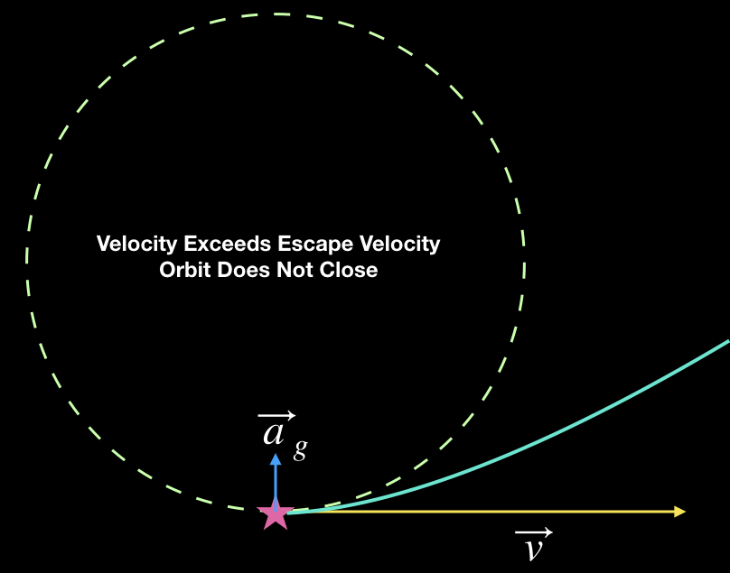
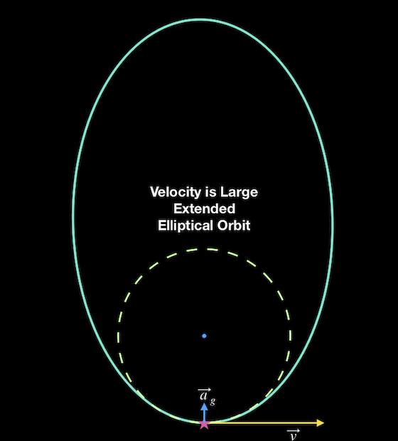
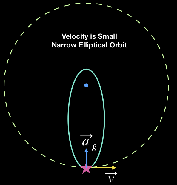
In the schematic diagrams above, the dotted green circle is understood to have a constant size. It represents the orbit of an object with a set of orbital parameters (energy and angular momentum) that will produce an orbit of that particular shape and size. The solid green curves are for orbits with different energy and angular momentum. These produce orbits with different shapes and sizes. The circular orbit is shown on each diagram to make comparison possible between the various other orbits. The velocity required to produce this circular orbit would lie somewhere between the “Large Orbital Velocity” and “Small Orbital Velocity” of the middle pair of examples.
The case just considered, that of zero orbital velocity, is an extreme case. In general objects do have some non-radial velocity component. Let’s imagine giving our test object a small nudge sideways. Now part of its velocity is not radial. What is the result of that? Well, the orbiting body will still fall toward the center, but as it does so it will move sideways, too. So it won’t oscillate along a line as described above. However, as it falls inward its original sideways velocity will begin to feel a stronger and stronger gravitational effect acting to slow it down. Eventually, its sideways velocity will stop completely. Thereafter the sideways motion will reverse. The upshot of its motion and the changing gravitational attraction (again, we assume that the gravitational acceleration is proportional to \(1/r^2\) ) will cause the test object to move faster and faster along its path, which will sweep closely to the massive central object and then arc out to the point at which it was first set in motion. It will have exactly its initial velocity when it arrives there, and so the motion will repeat this way indefinitely. The situation is depicted at top right, above. Notice that the orbit is now a narrow ellipse, so still not a circle, but not a line, either.
We can imagine giving the test object larger and larger sideways velocities to start out its motion. As we do this, the the arc it follows will broaden more and more as the initial (sideways) speed increases, and its closest passage to the central object (called perihelion for an object orbiting the Sun, say) becomes larger and larger. At some point the orbit will be a circle. That will happen when the initial sideways kick will be enough to exactly cancel the inward fall toward the center, and so the object will follow a path of constant distance from the center of the orbit, a circle, just as we imagined initially. Incidentally, a circle is still an ellipse, it’s just a special case, as well see below. The circular path is shown using a dashed pattern, and in each of the diagrams this circle should be taken as being identical in size to all the others. Its depiction has been altered so that the different orbits, which each have different sizes, can be shown in the various diagrams.
If we give a the body a larger velocity kick than this, then gravity will be too weak to counteract the sideways motion and keep it a circle. Instead, the object will move a small distance away from the center. In this case the orbit will again be an ellipse, but it will lie outside the initial circle. The object will eventually slow down, cease its outward motion and begin to fall back. In this case it will sweep back past the central object and return to its initial position. The orbit might look something like the path shown above at lower left. Finally, we could give the object so much velocity that it simply never comes back. In that case its energy of motion (kinetic energy) is larger than the energy in its gravitational attraction (gravitational potential energy) and the orbit will be a hyperbola. The orbit does not close back on itself, and the object leaves the system. That case is shown above at lower right.
There is a borderline condition on the orbit as well, the boundary between a closed orbits and an open ones discussed above. In this case the kinetic energy of the orbit exactly equals the potential energy. Orbits with this condition are parabolas. They are not closed, and in fact the object never falls back. Instead, it moves outward forever, slowing more and more as it does, and it approaches, but never quite reaches, stillness the farther it travels. These orbits differ from the hyperbolic orbits because in the latter, the motion of the object approaches a finite, non-zero speed as it moves farther away. These parabolic orbits appear quite similar to the hyperbolic ones, though they are narrower, and so there is no separate diagram shown for them.
We will look at the effect of energy on the orbit in greater detail in the next section.
You probably noticed that the elliptical orbits are offset from the circle. This effect is real: in elliptical orbits the center of attraction is offset from the center of the orbit. In the solar system, the Sun seems to be at the center, but this is only true because we generally only think about the planets, and they have near-circular orbits. For comets, which have very elliptical orbits, the Sun is nowhere near the center. It is offset and is located at one of the foci of the comet’s elliptical orbit. Ellipses have two foci, and nothing is located at the second one. As an ellipse becomes closer and closer to a circle the foci move closer together. Finally, for a circle they lie directly on top of one another. So even for a circular orbit the central object is at a focus of the ellipse, but in the case of a circle this happens to be at its center.
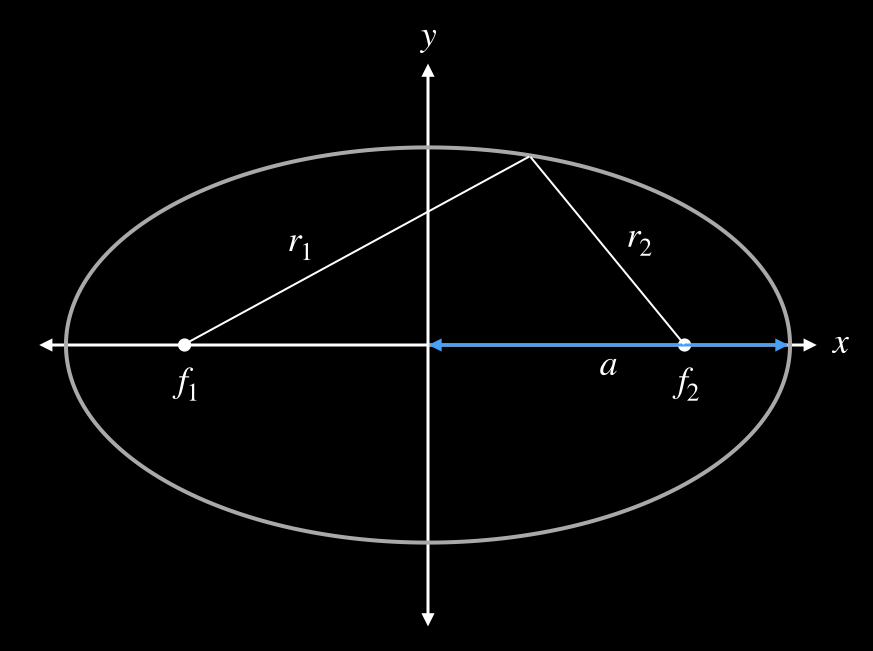
The diagram below shows an ellipse and its two foci, along with the geometrical relationships between the axes of the ellipse and the location of the foci. The curve is the set of points that satisfy the expression \(r_1+r_2=2a\) where \(a,\) shown in blue, is called the semi-major axis of the ellipse. It is half the distance across the longest straight path through the ellipse. If you consider this mathematical relationship for the case of a circle, where the two foci lie on top of one another, you will see that it is still satisfied, so a circle is indeed a special case of an ellipse.
In the solar system, the Sun is at one of the foci. Nothing is located at the other focus. This is typical for systems with a single dominant object. For example, the planets all have nearly circular orbits. That means the two foci lie nearly on top of one another, well inside the Sun. For objects with highly elliptical orbits, like the shape shown in the figure, the foci are quite distant from one another. These are the kinds of orbits followed by many comets and asteroids.
Of course, some objects are not bound to the Sun at all. They fall through the solar system on orbits that never loop back and return. Those orbits would be parabolae or hyperbolae, not ellipses. Their second foci are located an infinite distance away from the Sun. All of these shapes are allowed orbits in Newtonian gravity. They are called conic sections because they are the curves created by the intersection of a plane with the surface of a cone.
Orbits and Conservation Principles
The various cases outlined above can all be understood as expressions of two basic physical laws: the law of conservation of energy and the law of conservation of angular momentum. The first law states that the total energy of a system remains constant. The second says that the angular momentum of a system remains constant. Lets break these down so that we understand what they mean.
The energy of any object has two parts. One is the energy it has because of its motion. This is called kinetic energy. In the non-relativistic case (when speeds are not close to the speed of light) the kinetic energy of an object is given by the expression below. The kinetic energy is often represented by the symbol \(T,\) and that is how we will represent it.
$$ T = \frac{1}{2}mv^2 $$
The expression gives the kinetic energy of an object with mass \(m\) that moves with a speed \(v.\)
Lots of other types of energy are really just kinetic energy masquerading as something else. For example, the temperature of a gas is really just a representation of the average kinetic energy of the particles in the gas. While there is always a spread of speeds of particles, the faster the typical particle moves, the higher the average kinetic energy and the higher the temperature of the gas.
The second type of energy a system can have is called potential energy. Potential energy results from interactions between objects. So, for example, if there is an attractive interaction between two objects, like gravity, then there will be energy associated with that interaction. Since the strength of the interaction usually depends on the distance between the objects, the potential energy will change when the objects move either closer or farther from one another. For gravity, the potential energy is given by the expression below. Potential energy is usually represented by \(U.\)
$$ U = -\frac{GM m}{r} $$
The \(G\) in this equation is the gravitational constant, the same constant is we find in Newton’s Universal Law of Gravitation. Remember, it is there to keep track of the units of measure we are using (feet or meters for length, kilograms or slugs for mass, for example), and to give us some idea about how strong the gravitational interaction is. Beyond this it is not very important. In the SI system of units, \(G\) has a value of \(\rm{6.67\times10^{-11}\,N\,m^2\,kg^{-2}}.\) That is quite small, so gravity is only a strong interaction when very large amounts of mass are involved - or perhaps over very tiny distances.
Note that the potential energy related to gravity is always negative. This reflects the fact that Newtonian gravity always produces an attractive force. It is never repulsive. The negative sign for attractive forces is a convention, but it carries across to all branches of physics. For example, in contrast with gravity, the electric force can be attractive or repulsive. Two positive charges repel one another, as do two negative charges. Only when there is a negative charge paired with a positive charge is the force attractive. So the electric potential energy can be positive or negative, it just depends on the sign of the charges. With gravity, since there is only one kind of mass (there is no negative mass), the energy is always negative, and therefore by convention attractive.
Potential and kinetic are the only two kinds of energy there are. All forms or sources of energy that you have heard about are combinations of the two of them. For example, the energy in fuels like oil or wood are types of electrical potential energy. This energy is stored in the chemical bonds (interactions between electrons) in the fuel. The energy extracted by a dam to drive an electric generator starts out as gravitational potential energy. It is converted to kinetic energy as the water falls from the top of the dam to the bottom where the generator is located, and is finally extracted from the kinetic energy of the water and stored in the electric and magnetic fields of the generator - potential energy. Even nuclear energy is a form of potential energy, but in this case it is energy stored in the interactions between particles in the atomic nucleus, not electrons.
There are exactly four kinds of potential energy, one for each of the four fundamental interactions: gravitational, electromagnetic, strong nuclear and weak nuclear. Fortunately, to understand orbits in the solar system or in galaxies, etc., we only need to worry about gravitational potential energy. The other fundamental interactions do not play a role.
For an orbiting object, we can write an expression for its total energy, which is the sum of its potential energy and kinetic energy. The total energy is given below.
$$ E = T+U =\frac{1}{2}mv^2 -\frac{GM_1 M_2}{r} $$
Consider this expression. It provides useful (and quite general) insights into orbits and orbital motion. First, note that the total energy can be either positive, negative or zero. The kinetic energy is always positive, of course, because it is the product of terms that are themselves always positive. As we mentioned already, the potential energy for gravitation is always negative. We have three possible cases to consider, and only these three cases.
E > 0
The total energy is positive. The kinetic energy exceeds the (absolute value of the) potential energy.
In this case the energy of motion is greater than the energy of attraction, so the system is not bound.
The system will not be stable and objects within the system will generally follow paths that are not closed, as shown in the lower right diagram above.
E= 0
The total energy is zero. The kinetic energy exactly equals the (absolute value of the) potential energy.
In this case the energy of motion balances the energy of attraction, so the system is marginally bound//unbound.
The system is not really stable, as it will expand to infinite size in time. The paths of particles are not closed, as shown in the lower right diagram above.
E< 0
The total energy is negative. The kinetic energy is less than the (absolute value of the) potential energy.
In this case the energy of motion is smaller than the energy of attraction, so the system is bound.
The system is stable, and objects within it will generally follow closed orbital paths as in any of the three diagrams above, excluding the lower right diagram.
From the three cases above we see that the boundary between bound and unbound orbits occurs when the total energy is zero. This allows us to assign a specific value to what is meant by “Very Large Orbital Velocity” in the description of orbits. To do so, we set the total energy equal to zero and solve for the velocity.
\begin{equation}
\begin{split}
0 &=\frac{1}{2}mv^2-\frac{GMm}{r}\\
& = \frac{1}{2}v^2-\frac{GM}{r}\\
v^2 & = \frac{2GM}{r}\\
v_{esc} & = \sqrt{\frac{2GM}{r}}
\end{split}
\end{equation}
So this critical speed, over which an object becomes unbound, below which it is bound, is given by the simple expression above. It is important enough that it has a special name: it is the escape velocity. You can understand why it is so named by considering the following cases.
First, imagine you throw an object, say your keys, upward. You know they will rise, ever more slowly, until they finally stop. Then they will fall, increasing their speed as they fall. This slowing and falling is a direct example of the exchange of energy between kinetic and potential. You impart a certain amount of kinetic energy to the keys when you throw them upward. That kinetic energy is converted to potential as they rise, and when all of it has been converted they no longer have any energy of motion. They have stopped. Of course, gravity has not ceased its pull, so the keys begin to fall. As they do so, they lose potential energy, converting it into kinetic. The keys speed up. Energy is conserved.
Now imagine that you throw the keys a little harder. They have a bit more kinetic energy at the outset, so they must rise a little bit farther before it is all used up, converted into potential energy. They then fall back down and arrive back at the ground moving with their initial speed, but now going down instead of up. You can repeat the experiment over and over, giving a little more energy each time. As a result the keys will travel higher before they stop and fall back down. Is there a point at which you have thrown the keys so fast that they just never come back down?. If you have understood the derivation of the escape velocity, you will know that the answer is yes. If you throw the keys at the escape velocity - or at a higher speed - then they have so much kinetic energy that gravity will never be able to stop them and pull them back down.
For Earth, the escape velocity is about \(\rm{11\,km\,s^{-1}}.\) That is quite fast. Certainly it is faster than anyone could possibly throw a set of keys. However, it is not so fast that a rocket cannot propel objects fast enough to escape. But Earth is so huge, that even a giant rocket like the Saturn V could propel only a tiny capsule out of Earth’s immediate vicinity and send it to the Moon. Escaping from an even larger object, the Sun for example, is harder still.
So objects that travel at or above the escape velocity are not bound, and they escape out into space. But what happens to objects that move more slowly? They will be bound, but why then don’t they simply fall into the object attracting them? Why doesn’t the Moon fall into Earth? Why doesn’t Earth fall into the Sun? After all, the energy of gravitational attraction for these bound objects is greater than their energy of motion. Why doesn’t gravity simply pull them down into the center of their orbit? In short, it doesn’t because it can’t, at least not according to Newtonian gravity (general relativity, a more complete theory of gravity, says something else, but we will leave that to a different article).
Conservation of energy is important for orbits, but it does not alone determine them. Conservation of angular momentum also plays a vital role. It is conservation of angular momentum that prevents orbiting objects from collapsing inward, and that keeps them stable over time. Conservation of angular momentum is the subject to which we turn our attention next.
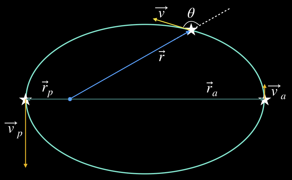
The diagram above depicts an object at three places along its orbital path. At left and denoted by \(p\) is the periapsis, the point of closest approach to the attracting body. For a body orbiting the Sun this is given the special name perihelion (after Helios, the sun god in Greek mythology), and for a body orbiting Earth it is called perigee (after Gaia, the Greek goddess of Earth). In any case, this is the point of an orbit’s closest passage to the central attracting object.
At right is the apoapsis, the point at which the object is at its farthest point from the central object. For objects orbiting the Sun this point is called aphelion, and for those orbiting Earth it is called apogee. Similar terms pertain for objects orbiting other stars: periastron and apastron. Collectively, the extreme points of an orbit are generically called the apsides (ap-si-dees), regardless of the body being orbited. These points in the orbit are important not just because they are the turning points, where an orbiting body changes from moving toward/away from its central object, but because they are the easiest points at which to determine the orbital angular momentum.
Angular momentum depends both on an object’s linear momentum, \(\vec{p}\), and its position, \(\vec{r}\). It is generally denoted by a capital \(\vec{L}\). The angular momentum of an object is always computed in reference to some particular point in space. For orbital motion, it is generally convenient to take as a reference the central object that is being orbited (like the Sun, for example), and that is what we do here. The blue dot in the diagram represents that object. All distances are measured from that point, and so all the radius vectors in the diagram start there. The velocities are all tangent to the orbit at the point where the orbiting body is located at the moment of interest. With these conventions in mind, the angular momentum can be computed in a consistent way using the expression given below.
$$\vec{L} = \vec{r} \times \vec{p}$$
In this expression, \(\vec{p}\) is the linear momentum, the product of the object’s mass and its velocity.
$$\vec{p} = m \vec{v}$$
From the notation we are using it is clear that \(\vec{L}\) is a vector. Its direction does not really concern us here, so we will not describe how it is determined. If you want to know, take a look at the blog post about why galaxies are disks. That topic is intimately tied up with the direction of the vector \(\vec{L}\), so we spend much more time discussing it there.
For our purposes presently, we are more concerned with the magnitude of the angular momentum vector, or in other words, its length. That is given by the expression below.
$$L =rp\sin\theta$$
The expression gives the magnitude of the angular momentum, \(L\), at any point in the orbit. In general, the values of \(r\), \(p\) and \(\theta\) will be different at each point in the orbit. To understand the expression, look at the diagram above, and consider the case when the object is between apoapsis and periapsis. Notice that the angle between the direction of the vectors \(\vec{r}\) and \(\vec{v}\) (the velocity vector is always tangent to the curve at the point of interest) is an angle we call \(\theta\). The angle \(\theta\) varies as the particle moves around its path, just as \(r\) and \(v\) do. The direction of \(\vec{r}\) is made more clear by extending it with the dotted line. The magnitude of the angular momentum, \(\vec{L}\), depends not only on the magnitudes of the position and velocity vectors, but on their relative orientations. If \(\vec{r}\) and \(\vec{v}\) are parallel (\(\theta = 0\)), or antiparallel (\(\theta = 180^{\circ}\)), then there is no angular momentum at all because \(\sin 0\,= 0\) and \(\sin 180^{\circ}\, =\, 0\). If \(\vec{r}\) and \(\vec{v}\) are perpendicular ( \(\theta = 90^{\circ}\) ), then the angular momentum is simply their product, because \(\sin 90^{\circ}\, =\,1\). That is the case at both the apoapsis and periapsis.
The important thing to understand about the angular momentum is that it is a constant of the orbit, meaning it does not change as the object moves around its orbit. This is true for both the direction of \(\vec{L}\) and its magnitude, but as we stated, we are presently only concerned with the magnitude. So in particular, consider the cases of perihelion and aphelion. The angular momentum must be the same at these points in the orbit.
\begin{equation}
\begin{split}
L_a &= L_p\\
r_a p_a & = r_p p_p\\
r_a m v_a & = r_p m v_p\\
r_a v_a & = r_p v_p\\
v_a &= \left (\frac{r_p}{r_a} \right ) v_p
\end{split}
\end{equation}
Have a look at the last line in the equations above. It says that the speed of the orbiting object when it is at apoapsis is smaller than its speed at periapsis in exactly the proportion that its distance at apoapsis is larger than its distance at periapsis. And of course, the same is true at all the other points in the orbit, with the caveat that at those positions we have to consider the angle \(\theta\) because it will not be \(90^{\circ}\) at those points, it will vary. What this means is that the object moves slowest at apoapsis, where it is farthest away, and it moves fastest at periapsis, where it is closest. At other points in the orbit it moves with some intermediate speed. But there is a limit to how small \(r_p\) can be because there is a limit on how large \(v_p\) can be. Certainly the velocity at periapsis cannot be so large that the kinetic energy at periapsis causes the total energy there to exceed the total energy at apoapsis. If it did it would violate energy conservation, an independently satisfied condition. The two conservation laws together place an absolute constraint on how close the object can come to the central gravitating object at its closest approach.
The momentum relations alone do not give us any information about the actual speeds at any point in the orbit, they just tell us how the speed at any given point compares to speeds at other places along the path. Similarly, the energy equations alone do not tell us anything about the shape of the orbit. That depends in detail on the orbital angular momentum. The two sets of equations together, however, along with the expression for the gravitational force (or equivalently, the gravitational potential energy), provide us with all the information we need to compute the exact orbit of the object.
The basic takeaway is that orbital motion consists of objects falling toward each other under the influence of gravity, but not usually merging because conservation of angular momentum keeps them from getting too close. Instead, they fall toward and then away from each other in a continuous cycle, exchanging kinetic energy for potential energy, over and over again. That is what an orbit is.
This article covers the basic concepts needed to understand orbits. If you are interested in seeing the mathematical details that go along with it, you should consult a book on celestial dynamics. An excellent one is called Fundamentals of Astrodynamics by Roger R. Bate, Donald D. Mueller and Jerry E. White. There is a Dover edition available. The mathematics required is not too difficult. One needs to know only what is learned in the first year or two of introductory college level physics and math courses. If you don’t want to trouble with that, then hopefully this short description will give you a better understanding of what orbits are and how they work.